Detecting clouds in satellite images using convolutional neural networksd

Convective clouds, as the name suggests, are clouds which contain a physical process called convection:

1. Warm air close to the ground is lighter than the surrounding air, so it rises.

2. As the air rises it cools, at a certain point it becomes heavier than the air around it and starts to fall again.

3. The air starts to warm again and the cycle restarts.

Convection is a very general process that takes place everywhere from a cooking pot to the surface of the sun, so let’s focus on how this looks in clouds specifically.

First, moisture evaporating from the surface of the land or sea forms what’s called a cumulus cloud. If the cloud is warm enough compared with the surrounding air it will continue rising and become a towering cumulus (TCU) cloud. At this point convection starts inside the cloud.

If the cloud can continue rising it will eventually reach what is called an inversion. This is a point when the air starts to get warmer as you rise rather than colder. The cloud can’t rise any further than here so it starts to flatten out. It then becomes a cumulonimbus (CB). These are quite easily recognisable by their striking anvil shape.

CBs can generate extremely strong updrafts and downdrafts which can be dangerous for aircraft taking off and landing so it’s important to know where these clouds are. There are several different methods for convective cloud detection using weather radars or lightning strikes but in this series we will discuss the use of satellite images. The goal will be to take a satellite image from EUMETSAT and segment it into three areas, CB, TCU and no convective clouds.

The data we used is from two satellites Meteosat 10 and 11. These are in geostationary orbit above Africa (that is, they take a full 24 hours to orbit the earth along the equator, so that they remain above the same position on the earth’s surface). Meteosat 11 takes an image of the whole earth disk every 15 minutes and Meteosat 10 takes an image of the northern hemisphere every 5 minutes. This is because the satellite doesn’t function like a normal camera that records all pixels simultaneously, instead it spins, recording one pixel at a time before starting on the next row. Naturally this means that imaging a smaller subset of the disk is quicker than the entire disk. We crop and resample the image to just cover Germany so we can use either satellite image interchangeably.

Those of you who are especially interested in the technical aspects of the data we are using find the Meteosat Second Generation Level 1.5 Image Data Format described in great detail in this document.

A normal image is made up of three values, or channels: for each pixel red, green and blue. The relative values describe the colour of the pixel. However, if the main goal of the imaging is not for human viewing but to extract quantitative information, then there is no reason to restrict to only these three channels. This satellite data has 12 channels, described in the table below:

So we have a lot of information here! We are going to provide all of this to our model to make predictions.

We also need some labels in order to train a model. Unfortunately, this means human labelling! To do that we need to present the data in a format that makes the convective clouds stand out. The obvious starting point is to display the HRV channel.

This is a good start but there is still not enough information here to make a decision. One of the most useful measures is the temperature of the clouds since this is a good indicator of the height of the cloud top. We do this by overlaying the temperature information as a colour.

Finally, we can also provide the person doing the labelling with a radar image. There are a number of radar stations across Germany. Radio waves are reflected by water droplets, i.e. rain. This is very helpful because Cumulonimbus clouds normally produce a lot of rain. They can be very easily recognised in the radar image by the high intensity and gradient of the rain when compared to other rain producing clouds such as stratiform clouds.

Radar is mostly reflected by rain, so we can spot the characteristic small but intense areas of rain produced by convective clouds as opposed to the broader areas with lower gradients associated with the frontal system.

Now that we know how to label the CBs, let’s consider how we can label the TCUs. Cumulus clouds (whether towering or not) are actually quite easy to spot. They normally appear as large fields of small bright clouds.

We then have two difficulties: first that it would be impractical to label each cloud individually and secondly to distinguish the towering cumulus from the rest of the cumulus. Fortunately, we can use a bit of meteorology knowledge here. Towering cumulus clouds are higher and mostly made up of ice crystals rather than water droplets, hence they have a higher albedo (i.e. they reflect a larger portion of the light they recieve). Since the satellite measures the number of photons received, all we need to do to calculate the albedo is to estimate the incident radiation. Fortunately the sun’s output is fairly constant, so we just need the solar zenith angle which we can calculate easily from the time of day and year. Then we just need to find a good threshold value by hand to ensure that we separate the clouds correctly.

You can see that the CB clouds tend to be compact regions with high IR reflectivity and TCU tend to be smaller scattered clouds.

Having learned how to get labeled data we can now discuss how we will actually build a model to make our predictions.

At its core this is a semantic segmentation problem, i.e. we need to classify each pixel in the image into three classes: CB, TCU and no convective cloud. A number of different algorithms have been proposed for this class of problem, but the current state of the art is a neural network architecture called a U-Net.

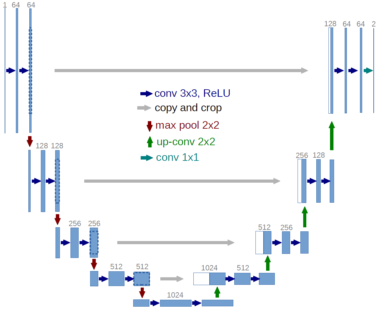
The U-Net is made up of a number of downsampling blocks followed by the same number of upsampling blocks. We have skip connections that connect points along the downsampling to points on the upsampling section. The idea here is that the later layers have access both to higher level features from the downsampled path and lower level features from the skip connection which preserve more local spatial information.
The original network was predicting two classes from a grayscale image, so it used one input channel and two output channels. We will be again predicting two classes but we will be using the twelve channel Meteosat image, so we will start with twelve channels rather than the one channel that the original UNET used.

We also made a number of other small changes to better suit our problem. We increased the number of recursions from 4 to 5 and replaced the up convolution with a pixelshuffle.

We now have our labelled data and a model. We now need to train it.

The raw data comes in 1024 by 1024 images which is quite large, in fact so large that we would be restricted to very small batch sizes if we trained on the entire images. If we downsampled the images we would lose the information contained within the HRV channel so we split the image (and the label) up into 16 smaller images of size 256 by 256. This lets us use rather large batch sizes ~64 images so we can really take advantage of techniques such as batchnorm and use very high learning rates to train models quickly.

We use a few tricks to get the most out of our data:

• First data augmentation. Normally when training a convolutional neural network on satellite images we can use any orientation of the images but here we have a disadvantage because the satellite is at a fixed position relative to the surface of the earth. This means, for instance, that cloud shadows will always appear slightly to the south of the cloud. We can only use a limited number of data augmentation techniques as a result. We used random horizontal flips and rotations of up to 10 degrees.

• One cycle learning rate annealing. We start with a very low learning rate and linearly increase it up to a maximum value (0.01 seemed to perform well) over the course of training before linearly decreasing it back down. This gives us the advantage of the slow learning rate “warm up”, a high learning rate to speed up training and a tail with a low learning rate to fine tune during the end.

• Mixed precision training. This is not possible on older GPUs, but allows us to save memory and therefore allow us to use larger batch sizes without sacrificing accuracy.

Finally we can produce and visualise a real prediction from the model:

Here we’ve marked CBs in blue and TCUs in green. You can see that we’ve correctly classified the large round CB clouds without incorrectly labelling too much of the frontal system (this is a common failure mode of existing non deep learning approaches). We’ve also correctly marked the small TCU clouds. 

If you want to read even more about this topic, we also did a project where we automated the detection of convective clouds for Deutscher Wetterdienst (DWD).