Collaborative Filtering in Recommender Systems

The goal of a collaborative filtering system is to infer how a user might interact with some item based on how other users with similar tastes interacted with this item. The similarity between users can be expressed in different ways and also can take into account different features of the users. In the context of purely collaborative filtering, which we will consider in this article, users are described only by the way they interacted with the items.

There are many interesting ways how one might formalize this mathematically and we will have a look at some of them. But first, let's have a closer look at the dataset we will be working with.

The MovieLens100k dataset consists of 100.000 user-movie rating pairs from 943 users on 1682 movies. In its raw form, without information about the users and movies, it looks like this:

As is very often the case with such datasets, most movies have very few ratings and most users have only rated a very small amount of movies.

As we can see from the plots in the above figure, most of the movies have a small number of ratings and likewise, most of the users have rated very few items. This is very common in recommendation systems. Notice that there are 1586126 ( = 943 * 1682) possible user movie interactions, however, only 100k of those have a rating - that's only ~ 6.3 %! The fact there is a handful of movies that get most of the ratings and that there are many movies with only very few ratings is also referred to as the long tail phenomenon.

Another way to phrase it is to say that the user-movie matrix is very sparse. With larger datasets, the following plot would not be feasible, but with the moderately sized dataset we are working with we can have a look at the user-movie matrix.

Here the rows represent the movies and the columns the users. The entry (or the pixel) at position $$(i,j)$$ is colored according to the rating that user $$i$$ has given the movie $$j$$. Or it is white if the user has not rated this movie. We can also have a look at a little patch, which is maybe more pleasing to the eye.

The images confirm the initial observations about the sparsity of this matrix. Another interesting thing to point out is that there are visible correlations between the columns and the rows of the matrix. This makes sense intuitively, as there are movies that simply are good (and hence receive mainly good ratings) - this explains the similarity between the rows. Also, some users tend to give better ratings than others - this explains the correlations between the columns.

In the case of purely collaborative filtering, the task we want to solve now is to predict how each user would rate each movie - and hence the missing entries in the user-movie matrix.

Train Test Split

To evaluate the performance of the algorithms, we need to create a hold-out test set. Ideally, we would want each user and each movie to be present in both the train and the test set. But since there are movies that have only been rated once, this is not possible. We will therefore sort out the rarely rated movies and create a split with the property that each user and movie which appear in the train set also appear in the test set.

Unfortunately, that way only 1541 movies (of 1682) remain in our dataset. However, for the movies which got sorted out, it would have been very difficult to make meaningful predictions anyway, and with the data available we also could not have evaluated these predictions properly.

Evaluation

So, how are we going to evaluate the predictions? Note first, that most common strategies phrase the prediction of ratings as a regression problem - that means, that the output of our models will be a continuous variable, even though the ratings are discrete (ranging from 1-5 only). For regression problems, typical evaluation metrics are the MAE (mean absolute error) and the MSE (mean squared error), as well as the RMSE (root mean squared error). Another typical metric for regression problems is the R² - score, which loosely speaking describes how much of the variance in the data is described by a model. Strangely, it does not seem to be widely used in online resources about the MovieLens100K dataset. In this blog post, I will focus on the RMSE only, as it is the most widely used metric with this dataset, but in the notebook, I report all 3 metrics. In case you are not familiar with the RMSE: It puts a higher penalty on larger deviations from the ground truth and is more forgiving with small errors. In general, one can say that the lower this metric is, the better and an RMSE of 0 indicate a perfect fit of the data.

Baseline

To have something to compare our results to later on, let's start with a very simple and unpersonalized baseline - for any unknown user-movie pair, we predict the mean of all ratings that other users have given this film. In the end, when we turn these algorithms into recommendation engines, this would correspond to just recommending the best-rated movies.

The user-movie matrix produced by this approach looks rather boring, as by construction all the rows are the same. Let's still have a look at it as it looks kind of pretty:

Evaluating on our test set we get the following metrics (note that we have calculated the mean values on the training set only).

• RMSE: 1.022

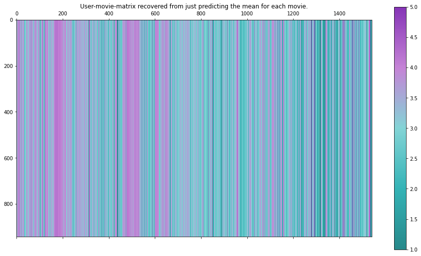
This approach is not the smartest. We have not considered any information about the users at all, so we cannot expect personalized recommendations. The rank of this user-movie matrix is one, as all columns are constant!

Just out of curiosity, we may do the same for the users. Note, however, that from a recommendation engine perspective this is useless, as by construction for each user all movies will have the same rating. We obtain the following metrics:

• RMSE: 1.042

As we will see later, these metrics are not too bad. This illustrates an important challenge in evaluating recommendation systems, as both approaches are basically useless in providing personalized recommendations but still give decent results when evaluated with these metrics. The first approach however is quite common when there is simply no information available, i.e. when a new user signs up for a streaming service!

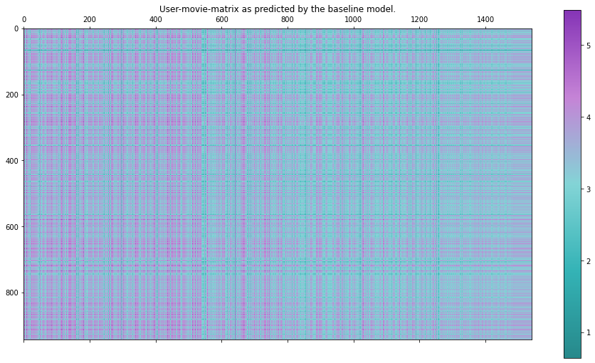
The algorithm, that is proposed as a baseline from the surprise library is a bit more sophisticated. For each user and each item, it introduces a (scalar) bias, $$b_u$$​ and $$b_i$$​​, respectively. These biases are learnable parameters. The prediction is then defined as

where $$\mu$$ is the mean of all given ratings on the train set. The parameters are learned via gradient descent on the training set.

This matrix looks much more diverse than the two previous ones and the metrics are better as well. However, the correlations between the rows and the columns are still clearly visible, which makes sense as they reflect the learned biases for each user and item. Note also, that from the perspective of personalized recommendations this approach is again "useless" - the ranking of the movies is still the same for each user, as it depends only on the learned movie biases $$b_i$$.

Evaluating on the test set, we get the following:

• RMSE: 0.944

Let's take a look at the distribution of the ratings as well. The left plot is a histogram of all 1541*943 predictions made by the baseline model, while on the right we only see the ~100k ratings for which we have ground truth.

The distribution on the left looks quite gaussian with the mean being close to the mean of all ratings on the train set. However, the model is rather hesitant to predict the "extreme" values 1 and 5 - this can be seen on the right plot in particular. Looking at the formula it makes sense that most predictions are very close to the mean and also that the extreme values are rare because for the rating to be very low (or high), either the movie or user bias should be very low (or high), which in term would lead to more other ratings being low (or high).

Let's start with the first "real" algorithm now. I chose to present an algorithm based on kNN (k nearest neighbors), as I think it is the most intuitive one and reflects the spirit of collaborative filtering in a very obvious way. It goes like this:

For a given user-movie interaction, find the k (this is a hyperparameter of this algorithm) nearest neighbors of the user (a.k.a. the most similar users) who have also rated this movie. Take the weighted average (weighted by the similarity of the other users with this user) of the ratings of the found users for this movie - that is the prediction. One formalizes the notion of nearest neighbors or most similar users by introducing a similarity measure $$sim(u, v)$$, which is high if the users $$u$$ and $$v$$ are similar. A typical and intuitive similarity measure is based on the euclidean distance - users are more similar if their euclidean distance is small. To put it in a formula again: The distance is given by

where $$I_{uv}$$ is the (possibly small) set of items rated by both users $$u$$ and $$v$$. The similarity can then be defined as

where the 1 in the denominator is present to avoid dividing by 0 and to bound this quantity from above by 1. Another widely used similarity measure is cosine similarity.

As we don't have further information about the users in our setting, we characterize each user with the vector of ratings he has given. So each user is identified with a vector $$u_i \in \mathbb{R}^{1541}$$, as we have 1541 movies in our filtered dataset. Recall, that for most of the users most of the entries of this vector will be empty. So to search for nearest neighbors means to find vectors that are most similar to the vector of the given user.

The formula for the prediction is

where $$N_i^k (u)$$ is the set of (at most) $$k$$ neighbors of user u, who have also rated the movie $$i$$ and $$sim(u, v)$$ is the similarity measure described above.

So let's have a look at what results this approach gives us!

• RMSE: 0.981

Here we chose to take into account the 40 most similar users (if there are that many) and chose the similarity measure based on the euclidean distance defined above. The cosine similarity produces much worse results, this is however readily explained/illustrated with the extreme example, where two users have only one rated movie in common, but one gave it the best rating (5) and the other one the worst rating (1). Since the cosine similarity normalizes the (in this case 1 dimensional) vectors to the unit norm, they turn out to be most similar - which is the total opposite of what we want in this case! This can be remedied by centering the ratings around 0, e.g. by subtracting 3 from all ratings. The results that this gave, in this case, were still slightly worse than the ones reported (which use the similarity measure based on the euclidean distance), so I will not report them here.

Notice that, especially in the right part of this matrix, there are many little white dots - in total there are 3460 of those. These correspond to user-item pairs, where the algorithm had too little information to make a prediction. So even though there might have been other users that rated this particular film, they did not have a single other film in common with this user, so there was no way to compute similarities and hence the user did not have neighbors in this space.

This is a major drawback of neighbor-based algorithms in such sparse scenarios. An obvious remedy would be to just predict the mean of this movie or the global mean of all ratings in such a case. Finally, let's have a look at the distribution of the predicted ratings.

Notice how there are remarkable spikes around the integers in the left plot. They are an artifact caused by the sparsity of the data and the design of the algorithm. For many user-movie pairs, there will only be one neighbor who has also rated this movie, and hence his rating just gets copied.

To remedy these weaknesses of the naive kNN algorithm, one can also take an underlying baseline (for example the mean rating) and fit a kNN model to improve this baseline. The formula then becomes

where $$b_{ui}$$ is the baseline prediction, which could depend on both user and movie, but doesn't have to. When choosing the baseline as the mean rating on our whole training set, i.e. $$b_{ui} = \mu$$, we obtain the following metrics and pictures:

• RMSE:0.954

Notice how suddenly the range of the predictions increased drastically and the model outputs values as high as 7 and as low as $$-1$$. This is because the formula involves another addition now and does not only take averages of already existing values, as our previous algorithms did. We can easily fix this by clipping the values at 1 and 5.

Overall, this variant:

• made our evaluation metrics better

• produced a more diverse user-movie matrix

• got rid of the problem of not being able to make a prediction (as the mean is the default prediction in this case)

Taking the baseline defined above as a baseline for the kNN algorithm improves the metrics even more:

• RMSE: 0.934

As the images corresponding to this approach are very similar to the previous one, I will not include them here.

Let's now explore a different family of successful algorithms for collaborative filtering - those based on matrix factorization.

We already observed that the columns and the rows in the user-movie matrix $$M$$ are likely to be correlated. In more mathematical terms, this means that this matrix probably does not have full rank. Algorithms based on matrix factorization exploit this fact by factoring this matrix as a product $$A \in \mathbb{R}^{943 \times k}$$ and $$B \in \mathbb{R}^{k \times 1541}$$ such that $$M \approx AB$$.
$$k$$ is a free parameter here and is typically chosen much smaller than the dimensions of the user movie matrix. By construction, the rank of the factorized matrix will be at most $$k$$.

Another thing that we get for free from following this approach is embeddings - a very fundamental concept in data science and machine learning.

The matrices $$A$$ and $$B$$ can be understood as collections of vectors of length $$k$$ - embeddings of the users and items in a joint vector space $$\mathbb{R}^k$$. By construction the interaction between user $$i$$ and item $$j$$ is then modeled as the dot product of their respective embedding vectors - it holds that $$M_{ij} = A_i \cdot B_j$$ .

In the literature and the surprise library, this approach is cataloged under the name SVD (singular value decomposition), as it is based on this concept from linear algebra. Let's try it out!

SVD Algorithm

• RMSE: 0.944

Let's have a look at the full user-movie matrix again. Note that the predictions may lie outside of the range $$[1, 5]$$ again so we clip them appropriately.

Notice how in our predictions some movies have a consistent scoring between different users, as well as some users that give consistent good (or bad scores) across different movies. That's a pattern we were able to observe in the sparse training set as well and it also makes sense that some movies are just good and some people just like all kinds of movies. :)

The influence of the embedding dimension

In our matrix factorization, we chose $$k = 100$$, so we assumed that the user-movie matrix has (at most) a rank of 100. A lower rank means that the rows and columns are more correlated, meaning that there is less variance between the ratings of the users or movies, respectively. Let's see how our metrics perform if we choose different values of $$k$$.

By choosing a larger $$k$$, we make the algorithm more powerful, hence it can achieve a lower RMSE on the training set. But the error on the test set is hardly affected by this - it is the lowest for $$k = 30$$ and we can achieve competitive results with $$k$$ as low as 15! So it looks like the choice of $$k = 100$$ was way too large.

Running the algorithm again with $$k = 30$$ gives the following results:

• RMSE: 0.951

The images and rating distribution are very similar to the case with the larger embedding dimension so I will not show them here.

The algorithm we used now corresponds to a technique known as probabilistic matrix factorization. We just (stochastically) factorize the user-movie matrix and take the entries of the resulting matrix as predictions. The surprise library also offers variants of the SVD algorithm, which tries to improve on an existing baseline model. However, since the results were not significantly better I will not include them in this, already quite long, blogpost.

Deep Learning

It is of course also possible to approach recommendation systems with deep learning. In the context of collaborative filtering, and in particular, with a dataset this small, this turns out not to be too effective. In the next article, where we cover content-based filtering, there will be many interesting deep-learning algorithms to consider.

I would like to briefly illustrate how we would now turn any of the considered algorithms into an actual recommendation system. In this purely collaborative setting, where we don't have further information about the users and the items, this will probably not be too enlightening but it is still a necessary building block.

We have to do two things:

• For a given user, filter out the movies he has already rated

• sort the predicted ratings descendingly, and return the top n (say, n = 5) movies.

Assuming that we have a model which also holds all the interactions from the training set and we can extract the prediction from a model for a given user-item pair with the get_estimate method, the code for a class that does this could look like this: (Check out the linked notebook for the actual code):

We can now sample some random users and have a look at their top 5 recommendations.

Recommended movies for user 792:
[603 233 296  52 643]
Recommended movies for user 846:
[603 233 296 512  52]
Recommended movies for user 498:
[512  52 437 296 233]

Some movies appear in all three selected recommendations, and some in two of them. This could be a coincidence, but let's check how they are rated in the training set.

So, these just seem to be popular movies that were rated by quite some people. The mean rating of movie 233 is not too high, however, a look at the histogram below reveals that it is generally well-rated in the training set.

To get a feeling for how diverse the recommendations are, we can compute the top 5 recommendations for each user and analyze them. In total, only 72 movies (out of the 1541 total movies) are recommended. Let's explore how often each one of those is in the top 5 recommendations for some users.

So apparently our recommendation system happily recommends the movies with IDs 233 and 603 to almost every user. As these are probably very popular movies, this makes sense.

What's cool, is that there are also quite some movies that get recommended between 10-50 times. What I also find interesting is the movies that only get recommended one or two times. It would be really interesting to explore if they make "sense", i.e. if they are in some sense similar to the movies a given user has rated well. But since we don't use information about the movies, this is not possible for now.

So far we have framed the problem as a regression problem. Also, the metrics we used for evaluation are prevalent in a regression setting. This makes a lot of sense for at least two reasons:

• The predicted variable has a clear interpretation. A higher rating simply means that the user is more likely to enjoy the movie more.

• When turning these algorithms into actual recommendation engines, recommendations naturally come with a ranking - there can even be items rated higher than the actual possible maximal rating, as we have seen.

However, it is still interesting to evaluate the performance on our test set as if it was a classification problem. We simply round the predictions to the next natural number and then take a look at the confusion matrix.

A few interesting things can be seen from this confusion matrix. First, our model has made all kinds of errors on the test set, except for predicting a 1 when the real label was a 5. That is quite good news, as this is the worst kind of mistake (together with predicting a 5 when the ground truth was a 1, which happened 10 times). The most frequent type of errors are confusions between 3's and 4's and 4's and 5's, respectively. These errors are not so bad, as they still reflect the general preferences.

Before we conclude this article, let's compare the different algorithms in terms of the RMSE (root mean square error).

What I find particularly interesting, is that the baseline model with only one learnable parameter per user and movie (so 943 + 1541 = 2484 parameters in total) is actually better than some of the kNN-based methods and also very close to the performance of the actual "best" model. This "best" model (out of the models we considered, on this specific test set) is the kNN-based model which aims to improve on the baseline. I'm writing best in quotation marks here because it is very hard to measure the success of a recommendation system with an offline metric. Offline in this case means, that the evaluation is carried out on historical data instead of in a live setting.

Usually, recommendation systems in production are hybrid models, which means that they are an ensemble of many different models. To compare different ensembles, companies use A/B testing: In a live setting, some users get version A and some version B. By comparing certain business metrics like click rates or conversions, it can be measured which system is better.

So, to conclude this blog post, let's summarise the main points.

We have

• introduced the concept of collaborative filtering,

• explored some purely collaborative approaches on the MovieLens100k dataset, in particular

  • a baseline model,

  • some k-nearest neighbor (kNN) based models,

  • an algorithm based on matrix factorization,

• converted one of these algorithms into a real recommendation system and explored its recommendations,

• compared the different models in terms of some offline metrics,

• and discussed how the evaluation of recommendation systems is a tricky thing.

I hope this blog post has given you some insights into the inner workings of collaborative filtering algorithms. In the next article, we will explore the concept of content-based filtering. Thanks for reading!