Visual Transformers: How an architecture designed for NLP enters the field of Computer Vision

We first recall the basic building blocks of the Transformer. If you are already familiar with the architecture, feel free to skip to the next section.

Encoder / Decoder

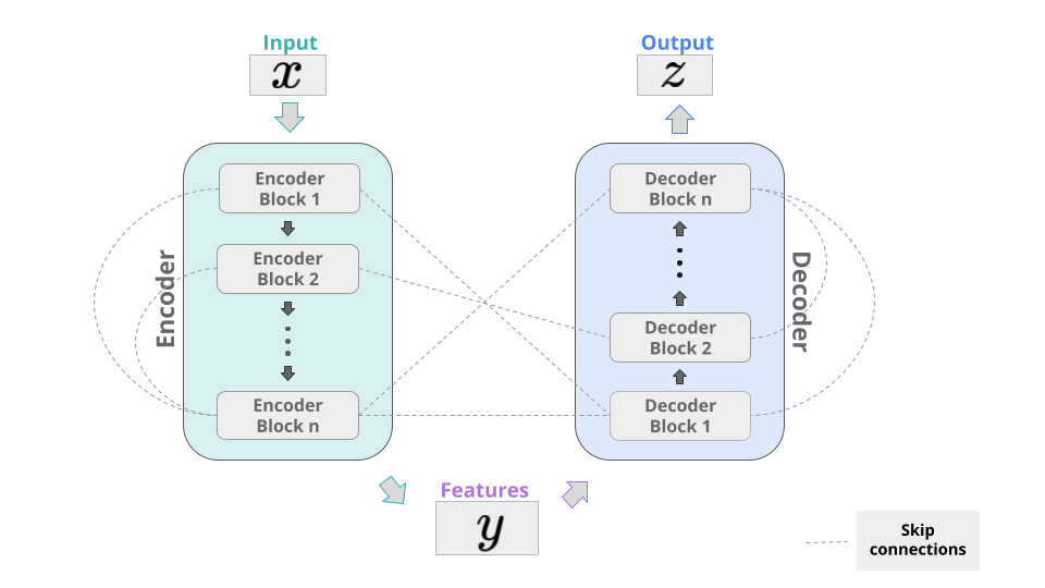
Like many other successful deep learning models, the Transformer consists of an encoder and a decoder part. The general idea is to encode some features of an input vector and then map those features to some output, decoding the relevant information from them. By connecting different layers through skip connections, the resulting model has more information available at each layer and one prevents the problem of vanishing gradients as well. In the Transformer, the encoder and decoder consist of a number of identical blocks, which rely mainly on the attention mechanism. The examples which we will cover here, like the famous BERT-model, only use the encoder part.

Attention

The self-attention mechanism is the heart of the success of the Transformer. It allows the model to understand which parts of the input are important and how relevant each part of the input is for other parts. Conceptually, a self-attention layer updates an input sequence by incorporating global information about the whole sequence for each entry. What makes it so efficient, is that it does not do this in a sequential manner but rather all at once. So like LSTM-networks, the Transformer makes it possible to naturally model long-range dependencies. However, as opposed to them, it is suitable for parallelization and hence allows efficient implementations.For an explanation how the attention mechanism is computed, check out this excellent blog article, our webinar on neural language models or the already mentioned paper Attention is all you need.

Tokens / Embeddings

Transformer-based models in NLP, like BERT, have a fixed vocabulary. Each element of this vocabulary is called a token. The size of this vocabulary may vary from model to model. For the BERT-base-uncased it consists of 30,522​ tokens. Notice how in the code example below some words get split up by the tokenizer. For different models, the input might get tokenized in a different way. In this code snippet, we import a BERT model from the great huggingface transformers library.

These tokens get mapped to vectors in a high-dimensional vector space (768 or 1,024 are common choices for the embedding dimension) by the embedding layer, which is learned during the training of the model. While propagating through the following encoder blocks, the resulting vector representations get updated through the attention mechanism or variants thereof (like multi-head-attention) and establishing context.

In the case of images, which already come with a numerical representation, the embedding layer gets obsolete and one also does not need to worry about a fixed vocabulary size. However, there is still a lot of ambiguity how to turn an image, which is typically represented as a matrix, into a sequence of vectors. We are now going to look at a few different ways to do this.

Before we have a look at the process of tokenizing images, let's start with a short digression on convolutional neural networks (CNNs).

The pixel-convolution paradigm

A common and so far still very successful technique in computer vision, is to apply convolutional layers to an image and create so called feature maps. Famous models like the ResNet and its successors follow this approach. Typically, one iterates this procedure in the following way: Suppose the input is an image in $$\mathbb{R}^{512 \times 512 \times 3}$$, that is an image of size $$512 \times 512$$ with $$3$$ colour channels. In a first step one might apply $$8 \ (3 \times 3)$$ convolution kernels so that the output is in $$\mathbb{R}^{512 \times 512 \times 8}$$ (the exact size of the feature maps may differ by a few pixels, depending on whether or not we decide to pad the edges of the image). In a second steps one could apply $$16 \ (3 \times 3)$$ kernels with techniques to reduce the dimensionality (like pooling), so the output would become an element of $$\mathbb{R}^{256 \times 256 \times 16}$$. The general consensus is that as the depth of the network increases, one should add more and more feature maps of ever smaller size.

The common view is, that feature maps deeper in the network represent more high level features, like shapes of some specific object, while feature maps closer to the input represent low level features, like edges. Although it has been shown that this approach of deep fully convolutional neural networks is very successful, it comes with 3 major drawbacks:

1. Every pixel is treated equally. What this means, is that convolutions process all image patches regardless of their importance and context within the picture. This leads to computational inefficiency, since often the relevant information is concentrated in a small part of a picture.

2. Most high-level features are only present in a small amount of images. Already the ResNet18, the 'smallest' version of this model, has as much as 512 feature maps at it's lowest level. For most images, probably only few of these feature maps are relevant for the output, however all of them are computed for every image which also leads to computational inefficiency.

3. It's not natural for a convolution to relate spatially distant concepts. By it's nature, a convolution only takes information from pixels in the vicinity of a pixel into account. By stacking multiple convolutional layers, information can slowly propagate through an image and techniques like larger kernels or dilated convolutions also make it possible to relate regions which are distant from each other. However, this results in a very large number of parameters and a high complexity, even if the task is simple.

To overcome this, the attention mechanism jumps in. Let's have a look at a few different ways how this can be done.

Tokenize by patching

A rather naive way to build tokens, is to simply chunk the image into smaller patches, flatten them into vectors and voilá - here you have your tokens. The Vision Transformer (ViT) does exactly this - with an additional transformation after the flattening to reduce the dimension of the tokens and a positional encoding, which is common for Transformers. The cool thing about this idea is, that it does not rely on different architectures (in particular CNNs) at all. So once again Attention is all you need. Concretely, the procedure works like this: Suppose that we have a $$512 \times 512$$ image with $$3$$ colour channels. With a fixed patch size of $$16 \times 16$$, this would result in $$N = 1024$$ patches. Now each patch is still a matrix (even a rank-3 tensor really) in $$\mathbb{R}^{16 \times 16 \times 3}$$ but we can simply stack all the entries in a vector of length $$16^2 \cdot 3 = 768$$ (which coincidentally also happens to be the size of the token embeddings in the original BERT model). The authors now apply a (learnable) linear transformation to reduce the dimensionality of the resulting sequence of vectors and obtain the tokens, this is however optional.

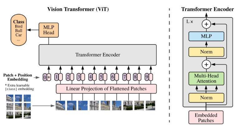
The creators of the ViT use it for classification, where only the encoder part is used and, like in the BERT model, a classification token is added. In the output layer, classification happens based on this token. Further applications include feeding the output through a decoder to perform regression tasks or segmentation. What is remarkable, is that the ViT does not utilize convolutions at all and still performs well on challenging datasets. This good performance however comes at a price: One needs really, really large amounts of data (and time, and resources), as it is common with Transformer-based architectures. The ViT was trained for image classification on the JFT dataset, which consists of over 300 million images, before being 'fine-tuned' on ImageNet with its 1.3 million images. For a detailed discussion about its performance on CV benchmarks be sure to have a look at the paper.

You can also find a ready-to-use, pretrained ViT in the transformers library.

Since relying only on transformers and attention is only possible with incredibly large datasets, let's have a look at how one can combine the approach with convolutions, to have the best from both worlds.

Generate tokens from feature maps

One such architecture is the Visual Transformer (VT), which should not be confused with the Vision Transformer (ViT)! It creates tokens in the following way:

First, convolutional layers are applied to extract some low-level features from the input image. Next, a tokenizer is applied to the feature maps to group the pixels into visual tokens. These tokens pass through a regular transformer to model relationships between the tokens. Their updated representations can then be used directly for classification, or they are projected back to the feature map to perform semantic segmentation. The most interesting part for me is how the tokenizer works, so let's check that out in some more detail.

The process consists of several steps. Given a set of $$C$$ feature maps in $$\mathbb{R}^{H \times W}$$ (height $$H$$, width $$W$$), one first flattens them and arranges them into a 2D matrix $$X \in \mathbb{R}^{HW \times C}$$. Now, a learnable matrix $$W_A \in \mathbb{R}^{C \times L}$$ is multiplied from the right to $$X$$ to form $$L$$ semantic groups. Applying a (row-wise) softmax operation, this yields a matrix, which carries a probability distribution over the $$L$$ semantic groups in each row (i.e. pixel of the original feature-map). By now multiplying the transpose of this matrix from the left to $$X$$, for each of the $$L$$ rows in the resulting matrix $$T$$, each entry is the weighted average over all pixels in the original feature map, where the pixels are weighted with their probabilities of belonging to the semantic group $$l \in L$$. This is illustrated in the below picture:

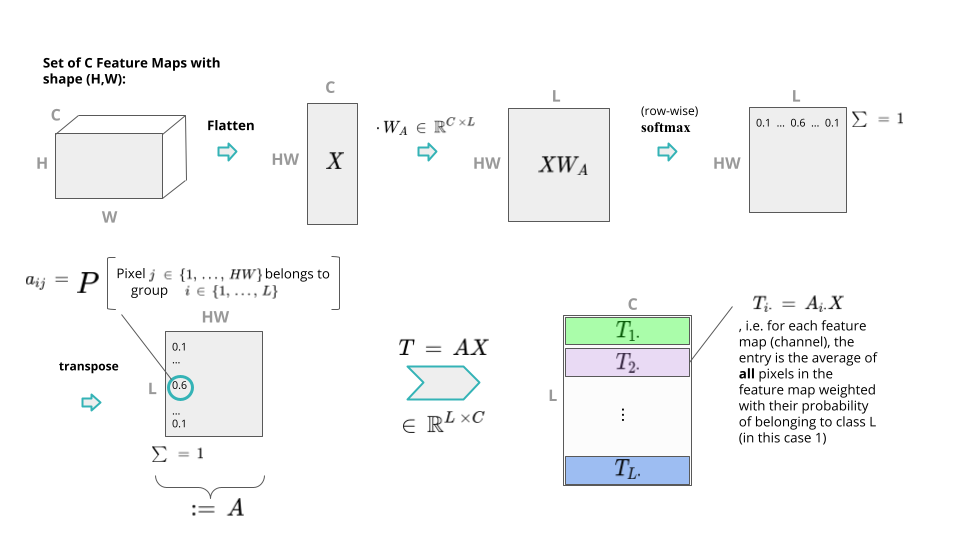
So, formally:

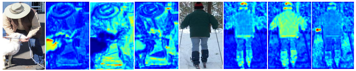
where the authors argue that $$L$$ can be chosen a lot smaller than $$HW$$ which reduces the complexity of the model. This process of tokenization is also referred to as computing spatial attention. By projecting the tokens back to their locations in the image, one can visualize what the semantic groups look like. Notice how different tokens highlight different semantic concepts in the images (red values are high, blue values are low).

In the presented experiments, the authors investigated the effect of the number of tokens ($$L$$) on the performance of their model. They looked at $$L = 16$$, $$32$$ and $$64$$ and, quite surprisingly, the performance increased only marginally with a larger amount of tokens. When using a ResNet-34 backbone to create the feature maps, the Top1 accuracy on ImageNet was even higher for $$L = 16$$ than for larger values. So indeed an image can be represented by a small number of visual tokens, at least so it seems.

The VT achieves great results on various benchmarks in computer vision, almost always outperforming its convolutional counterparts despite having fewer parameters. Compared to the Vision Transformer it needs very little time and data to train (it was only trained on ImageNet which still has over a million images).

For a more detailed evaluation of the performance be sure to check out the paper.

To conclude this article, let's recall the main points:

• Transformers were originally introduced to handle NLP tasks.

• For a long time (and until today), the standard tool in computer vision were convolutions. However they have their issues, like the problem to relate spatially distant pixels and 'over-complicating' some tasks.

• Together with convolutions, or even without them, the Transformer can successfully be applied to computer vision. When completely letting go of convolutions, enormous amounts of data and computing resources are needed.

• We had a look at 2 specific examples and what it can mean to tokenize an image.

• If you want to experiment with transformers in general, the huggingface transformers library is a good place to start. The timm (torch image models) package also offers implementations of transformers for computer vision tasks.

Of course we only scratched the surface of the applications of Transformers in this field. If you are curious about more, check out this survey on transformers in Computer Vision.