Migrating labels from Planet Scope to Sentinel-2

Moritz Besser

June 4th 2021

In this blog article, I want to briefly describe the process of migrating labels from Planet Scope to Sentinel-2 images. I will explain the process step-by-step and provide the necessary lines of code.

The code can easily be adapted to migrate labels between other satellites than in our example case here.

Introduction

One of the classic applications of machine learning has always been remote sensing. The sheer amount of data to analyze makes it a necessity to automate the process as much as possible. Illustratively speaking: one 100km² Sentinel-2 image consists of ~100 Megapixels which would take 5 hours to go through on a Full HD screen and 6 minutes per sector analysis. Imagine you want to keep track of urbanization processes in a country and therefore you are looking to detect changes in building footprints on satellite imagery. Instead of manually going through the footage to discover changes, you could create a training set consisting of satellite images and corresponding labels to train a neural network (NN) to detect buildings in the scenery for you. Or maybe you discovered a training dataset online which already covers your use case.

One problem you might face is that the labelling was done on a data source which differs from the satellite data that is available to you or a data source you want to use. So the image <> label combination has to be migrated or adapted to your sensor of choice. Some reasons why you might need to do that could be:

The satellite currently in use is decommissioned (e.g. Landsat 7 was supposed to operate until 2004 and still works, but might shut down suddenly at some point)
Higher accuracies are needed, so a higher resolution source will be used (e.g. going from 10m Sentinel-2 to <1m WorldView-1)
Transfer to another observation technology (e.g. switching from optical Sentinel-2 to radar (SAR) Sentinel 1)
Migrating from commercial to free sources (e.g. Planet Scope to Sentinel-2)

There are certainly more reasons to switch sensors, but regardless of the motivation, just the growth of possibilities to do so is impressive. This paper illustrates that fact quite nicely, as we can observe an exponential growth of operational satellites since the launch of the first earth observation (EO) satellite Landsat 1 in 1972.

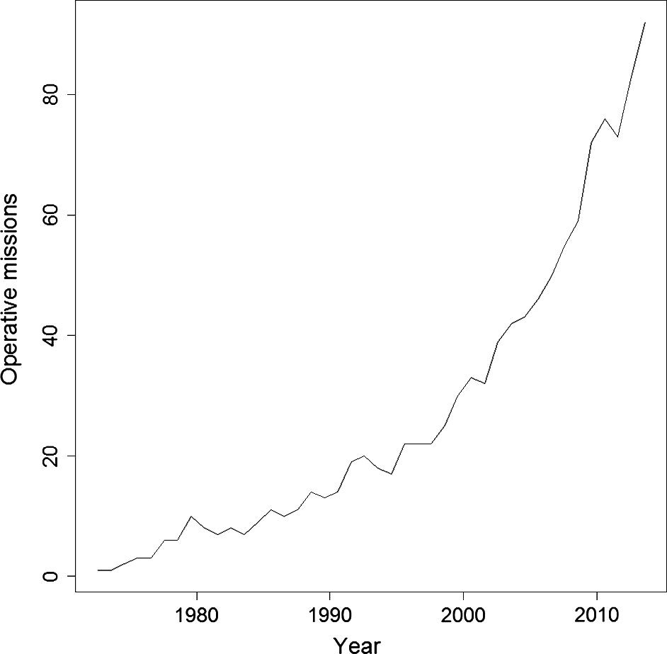
Graph showing development of number of operative satellite missions per year since 1972

Today (2021), more than 900 of such satellites are in service, therefore the trend even seems to be accelerating. The last point to motivate reusing labels is the fact that creating such labels is a work intensive and expensive process. Therefore: don’t relabel, but migrate!

Illustration showing that in AI most of the time is invested in getting labelled training data instead of coding

Getting started

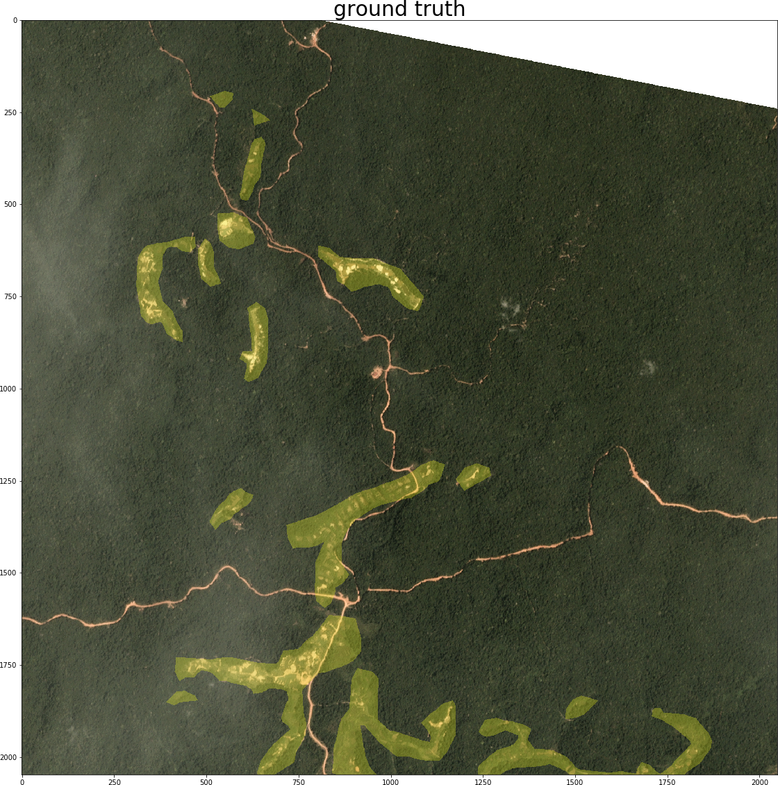
In this blog article, I want to briefly describe the process of migrating labels with references to our ASMSpotter to use Sentinel-2 instead of Planet Scope images. In that project we try to detect informal mining sites on rainforest satellite imagery. Here you can see an example of a mine mask (yellow) which was used in the training process:

Example of a mine mask (yellow) used in the training process

Our reasoning: while we had access to commercial satellite data during the development process, it might be possible to achieve similar results with free to use Sentinel-2 imagery. We had the hypothesis that in our case the additional spectral bands could compensate for the lower spatial resolution. The idea is simple: look for, download and crop satellite images of the new source to replace the images of the old source in the training set. For this method, the satellites obviously had to be operational at the same time.

One thing to note is that this transfer learning only works for more or less static objects which remain unchanged from one satellite image to another. Depending on the revisit times of the two sources, this can be hours to days or even weeks. So things like buildings, roads or vegetation cover would suggest themselves while vehicles, clouds and other weather phenomena most likely won’t work. In our case, we are detecting small open pit mines which are changing on the scale of months. Moreover, the new source ideally has a short revisit time to keep the temporal offset low.

	Planet Scope	Sentinel-2
spatial resolution	3m	10m
spectral resolution	4 bands	13 bands
revisit time	1 day	5 days

The most important thing though to check before thinking about migrating labels is the availability of geographic and recording time information. A problem of many freely available datasets is that they only provide the images and labels as ready to use pure image tiles (e.g. 256 x 256 jpegs) instead of geocoded and time referenced satellite images (like the GeoTIFF format). Those tiles aren’t really useful to us, as we have little chance to obtain the right corresponding observation for the new source. So, if you’re looking for datasets online, search for .tif files. Albeit missing detailed time information, this Inria dataset is a good example in the desired format.

Migrate it!

Now I will demonstrate how to migrate a label from a dataset towards Sentinel-2 (S2). As the Planet Scope imagery in our ASMSpotter project is proprietary, I’ll instead use data from the mentioned Inria dataset. So if you want to follow along with executing the code, download the dataset first. The steps we need to take for the migration are as follows:

create geocoded masks if not available (labels are called masks in image segmentation)
obtain new images
1. determine which images are needed for masks
2. download S2 images
3. convert S2 images to GeoTIFF
crop S2 image corresponding to original

Following are short code snippets for every step we take. We begin with the imports of our required modules:

from sentinelsat import SentinelAPI  # to download the new images

import rasterio as rio  # for all the GeoTIFF operations
from rasterio.features import dataset_features  # to load the mask
from rasterio import mask  # to crop the downloaded image
import imageio  # to read png masks
from cv2 import resize  # to resize the mask file
import geopandas as gpd  # to handle geographic information in GeoTIFFs

import pandas as pd  # to create dataframe with an image <> mask match
import os  # for file operations
from zipfile import ZipFile  # to unzip an archive
import numpy as np  # basic array operations
from datetime import datetime  # to extract recording date
from datetime import timedelta  # to create a time difference for the search

That looks like quite a long list. But actually it is only the API library to download the images, some packages to manipulate the images and some utility functions.

Step 1: Create geocoded masks

Now to step 1: the sample dataset actually contains geocoded labels already, so we can skip this step. As that might not be the case for your dataset, here is a short snippet to convert them:

# 1. create geocoded masks if not available
original_image_tif = 'path'
mask_png = 'path'

with rio.open(original_image_tif, "r") as src:
    # the important info is in the profile, so that is copied over
    mask_profile = src.profile      
    # we just have to update some info like bands count
    mask_profile.update({"dtype": "uint8", "count": 2, "nodata": 1})
    # now we read the png
    label = imageio.imread(mask_png)
    # in case there is 'no data' info, we have to carry it over
    no_data_mask = src.dataset_mask()
# now we just save the tif
with rio.open(mask_png + ".tif", "w", **mask_profile) as dst:
    dst.write(label, 1)
    dst.write(no_data_mask, 2)

You might ask why you would need to transfer the geoinformation from the images to the labels at all. Isn’t it enough to have it on the original footage and use it from there straight away? Yes, you’re right. There is no need to geocode the masks. But in an effort to make the dataset more easily migratable and shareable, I’d recommend to take this little extra step. This way it’s much easier to create a new training dataset for a new data source in the future: one only needs the labels, which is more compact and smaller than all the image-label pairs.

Step 2: Obtain new images

As we have the geoinfo already in the sample labels, we can go straight to step 2.1 to search for our new Sentinel-2 images. In the code I’m only using one tile from Vienna:

#  2.1. determine which images are needed for masks

# Sentinel-2 credentials
USER = 'put_your_user_name_here'
PASSWORD = 'put_your_password_name_here'

# specify the path and name of the mask file
mask_dir = 'data/AerialImageDataset/train/gt/'
mask_name = 'vienna36.tif'

# extract date from filename 
# (in our case its not present so we set it manually)
date = datetime.strptime('20210101', "%Y%m%d")
# get the area to look for from the geocoded mask file
with rio.open(mask_dir + mask_name) as src:
    features = dataset_features(src, band=False)
    bound_gdf = gpd.GeoDataFrame.from_features(features, crs=4326)
    area = bound_gdf.geometry[0].simplify(5)
# initialize the Sentinel API
api = SentinelAPI(USER , PASSWORD,
                  'https://scihub.copernicus.eu/dhus')
# check the availability of products for the mask
products = api.query(str(area),
                     # specify the time window around the mask date
                     date=(date - timedelta(days=10),   
                           date + timedelta(days=10)),
                     # there are different Sentinel 2 image types
                     producttype="S2MSI1C",  
                     # the smallest possible cloud cover should be used
                     cloudcoverpercentage="[0 TO 1]")
# keep track of what image belongs to what mask 
mask_s2_match = pd.DataFrame(columns=['mask_name', 'S2_name'])
for product_uuid in products:
    product = products[product_uuid]
    mask_s2_match = mask_s2_match.append({'mask_name': mask_name,
                                          'S2_name': product['title'],
                                          'S2_uuid': product_uuid,
                                          'cloudcover': product['cloudcoverpercentage']},
                                         ignore_index=True)
mask_s2_match.to_csv('mask_S2_match.csv')

You will need a login at the Copernicus Open Access Hub to be able to download the images, but you can quickly create one here. Two important settings are the date window and the cloud cover percentage: you want to keep both as small as possible, to avoid large differences between the original and the new image, which would decrease the accuracy of your labels. The best would be no clouds and same day imagery, but probably you have to make compromises between the two values depending on the data availability. For our example application of detecting building footprints we could easily use a large time window, as built-up areas only change over years. This way we have good chances of finding clear and cloud free images. When the API checks the available products for the mask, the results are saved to a csv file, so that we can keep track of the label and image relations. That is quite handy when we want to process big training sets.

Now we can proceed with downloading the products in step 2.2:

# 2.2 downlaod S2 images

# load the match file and select a product
mask_s2_match = pd.read_csv('mask_S2_match.csv')
product = mask_s2_match.iloc[0]

# download the selected product
response = api.download(product['S2_uuid'], directory_path='data/')

One thing to note is that footage older than 1 year is pushed to ESAs Long Term Archive (LTA). If you request such an image it takes up to 24h to get available again for downloading.

After downloading we have to turn the zip archive into a GeoTIFF in our step 2.3. You don’t have to dive deep into that bit of code, as it’s only the file format conversion and it is not necessary to adjust:

# 2.3 convert S2 images to geoTIFF

product_name = product['S2_name']
product_path = 'data/' + product_name + '.zip'

# unzip the product
with ZipFile(product_path) as zip_ref:
    zip_ref.extractall('')

# initialize
bands = {}
max_width = 0
max_height = 0
granule_dir = product_name + ".SAFE/GRANULE/"
jp2_path = granule_dir + os.listdir(granule_dir)[0] + "/IMG_DATA/"

# every file represents a band and has to be written to our GeoTIFF
for f in os.listdir(jp2_path):
    if f[-7:-4] == "TCI":  # skip this file as it is not a band
        continue
    band = rio.open(jp2_path + f, driver="JP2OpenJPEG")
    max_width = max(max_width, band.width)
    max_height = max(max_height, band.height)
    bands[f[-6:-4]] = band
with rio.open(product_name + ".tif", "w",
              driver="GTiff",
              width=max_width,
              height=max_width,
              count=len(bands),
              crs=bands["02"].crs,
              transform=bands["02"].transform,
              dtype=bands["02"].dtypes[0]) as dst:
    dst.nodata = 0
    band_names = ["01", "02", "03", "04", "05", "06", "07",
                      "08", "8A", "09", "10", "11", "12"]
    for i, band_name in enumerate(band_names):
        dst.write(bands[band_name].read(1), i + 1)
        bands[band_name].close()

Step 3: Crop S2 image corresponding to original

Now we can finally create our new training image matching the old label. Here is the code for step 3:

# 3. crop S2 image corresponding to original
match = pd.read_csv('mask_S2_match.csv').iloc[0]
mask_name, s2_name = match['mask_name'][:-4], match['S2_name']

# open mask and extract the boundary information
with rio.open(mask_dir + mask_name + '.tif') as mask_src:
    features = dataset_features(mask_src, band=False)
    boundary_gdf = gpd.GeoDataFrame.from_features(features, crs=4326)
# open s2 image
with rio.open(s2_name + '.tif') as s2_src:
    s2_crs = s2_src.crs  # crs stands for coordinate reference system 
    
    # crop S2 image 
    cropped_s2, tfm = mask.mask(s2_src, boundary_gdf.to_crs(s2_crs).geometry,
                                crop=True)

    # we have to update the new height and width information in the meta data
    profile = s2_src.profile
    profile.update(width=cropped_s2[0].shape[1], height=cropped_s2[0].shape[0])
    
    # save the cropped s2 image
    s2_cropped_path = open(s2_name + '_cropped.tif', 'w+b')
    with rio.open(s2_cropped_path, "w", **profile) as dst:
        dst.write(cropped_s2)

And that should be it! Let’s have a look at our results:

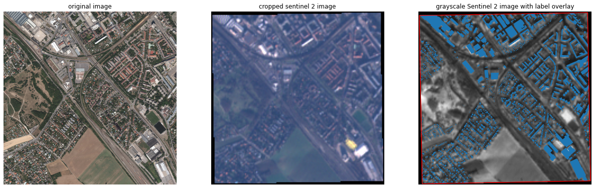
On comparing the left and middle images we can see that we’ve found the correct cutout. Also the ground truth in blue aligns nicely with the buildings in the grayscale Sentinel-2 image on the right. The black areas at the image edges are actually correctly blacked out. The red line depicts the area of the original image and as we can see it is not northed 100%. That results in the cropped Sentinel image covering a slightly larger area than the label provides data for, therefore we cover up those pixels in the image. A little note here: the code does not stitch together multiple Sentinel-2 scenes, so in case your label stretches multiple Sentinel-2 tiles you’ll have to adapt it.

Now you can just wrap all the code into ‘for loops’ to process all the old training labels and there you have your new training dataset.

Conclusion

We’ve achieved our goal of creating a training set for our type of sensor with little code and without the laborious labelling process. But there are things to keep in mind: most likely the training set quality will be degraded to some extent. Occlusions which are only present either in the original image or the new image will produce false negatives in the former and false positives in the latter case. For example, those occlusions can be produced by clouds in visual imagery or construction cranes in SAR (radar) data. Therefore, it is important to inspect the new dataset after migration and check the success of the process.

By the way, when we switched the training data from Planet Scope to Sentinel-2 in the ASMSpotter project we were first a bit worried about some wrong labels caused by cloud occlusion differences and expansion of the mines. But with a time window of +/- 10 days around the Planet Scope capture date, and a maximum allowed cloud cover of 3% for the new images, we found enough data to achieve almost the same f1 score in the new training process.

I wish you much success in migrating your own dataset!