How Google Cloud facilitates Machine Learning projects

Training a complex model on a sufficiently large data set can take days, sometimes months to do on a regular laptop, which no longer makes it a viable option neither when it comes to hardware nor time constraints. To mitigate these issues, dida makes use of Google's Cloud ML infrastructure, to be able to run long training sessions on customized, high performance, remote hardware which is independent of office hours, while simultaneously keeping local hardware available to our staff.

Even though training duration can be a bottleneck in some data science projects, it is hardly the only time-consuming phase. Although each project is unique with its own set of goals and challenges, there are certain recurring aspects of most data science problems that need to be dealt with again and again. Being able to automate and streamline some of these processes saves us time which can be spent on more fruitful things than merely configuring machine hardware and software.

The most reoccurring parts of our processes can be summarized as: 

• acquiring data,

• analyzing and pre-processing data,

• training a model on the data,

• and finally evaluating, visualizing and/or distributing the trained model.

Below, each process is described in further detail with hints and tips on how to speed things up using cloud services.

Most of the data sets we handle are text and image based. The former is usually relatively small in size, especially when compressed, which makes data transfer a rather trivial task. Image data sets however can be enormous, sometimes in the order of hundreds of gigabytes. Since some of us work remotely on laptops with limited storage space, downloading the data sets to a remote machine with an external 1 Gbps bandwidth is a great option.

Additional constraints such as download quotas and rate limiting are not uncommon. This often means that we have to distribute the images among the colleagues ourselves once downloaded from the source to stay within data cap limits. Cloud drives makes this easier, especially with persistent storage disks which are shareable between multiple Compute instances in read-only mode. Should read-only mode not be a viable option for the task, then there's always the possibility to connect the machines via the internal IP addresses. This yields network speeds between 2-32 Gbps depending on your CPU configuration, which is more than enough considering that read/write speeds on the standard Cloud Filestore SSDs are somewhere between 0.1-1.2 GBps (or 0.8-9.6 Gbps).

Data comes in many shapes and sizes. One thing that almost every data scientist has experienced is that raw data almost always fall into one or more of the following categories: badly formatted, incomplete, wrongly labelled, containing anomalies, imbalanced, unstructured, too small, etc. The old slogan "your results are only as good as your data" definitely has some validity. Therefore a lot of time can and will be spent on preparing the raw data, so that a model can be trained in a meaningful way. Click the link above if you're interested in learning more about some of the common pitfalls and how to avoid them.

A tool that caught our attention after attending the Google Machine Learning Bootcamp in Warsaw is the DataPrep tool, which makes handling Excel-like data a lot more convenient. The common way of handling unstructured tabular data is to go through each column one by one, looking for anomalies, misspelled duplicates, weird inconsistent date formats, and manually program a rule or exception for each one of these odd records. This quickly bloats the code base, is a tedious task and ends up being hard to generalize. DataPrep solves this problem more elegantly: with an intuitive graphical overview you can build so called "recipes" and apply them to your raw data source. These recipes transform your raw data step by step and output a clean table of data, which you can then pipe to your ML model, ready for training. If you are curious about how this works in more detail and have some minutes to spare, we recommend watching Advanced Data Cleanup Techniques using Cloud Dataprep from the Cloud Next '19 event.

After carefully constructing a model, it's time to train it using the data available. In the best of worlds, this would only have to happen once. However, as most data scientists have experienced, this is a highly iterative process, where hyperparameters are tuned, the model is refactored and optimized, loss functions compared and improved, etc.

Let's look at hyperparameter tuning for example. For any new hyperparameter introduced in the mix, time complexity can grow exponentially. Assume you have three hyperparameters to tune, let's say: learning rate, batch size and kernel type. If these all have four different values that you want to test, you'll end up having 4³ = 64 different combinations.

This is not much of an issue when the data set is small, a popular grid search cross validation method can often be performed on a laptop CPU over a set of hyperparameter permutations until an optimal combination has been found within a reasonable timeframe. As the model complexity and/or the data set grows though, things tend to escalate quickly. Suppose that one training session takes 24 hours on average to complete, which is not uncommon: then optimizing the hyperparameters mentioned above would need more than 2 months of training time.

So what are the options then? Since we might not be able to decrease the amount of hyperparameters that we need to test, the remaining option is to try to shrink the 24 hour training sessions down. Here, vertical and horizontal scaling comes to the rescue, in other words, increasing memory and processing power as well as parallelizing the computations on multiple machines. This is possible because when we look at what kind of calculations are done under the hood, it turns out that most neural network architectures can be represented as matrices. The multiplication- and addition- operations that are performed on these matrices can be done on a GPU. In fact, that's what a GPU is optimized for, because matrix multiplications are also the most common task when it comes to rendering graphics.

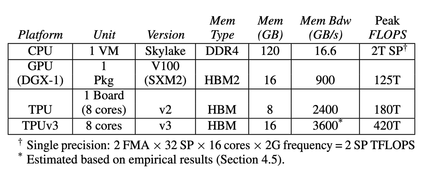
Today ASICs like the TPU, which are custom built for these types of operations, offer even higher performance. Wang, Wei and Brook at Harvard University performed a Deep Learning benchmark on the latest hardware configurations available in Google cloud, shown in the table below, and the winner is quite outstanding. GPUs performed over 60 times and TPUs over 200 times more computations than their competing CPU per unit time. In our example above, the duration of the hyperparameter tuning could be reduced from ca 2 months to about 8 hours. Although different tasks might see less benefits from these hardware options in terms of computational speed, that level of performance gain is hard to ignore.

Therefore we rely on the Google Compute infrastructure, where every employee can configure the hardware of a machine, tailored for his/her specific needs. Hardware options change all the time, but if you're interested in the specific options available right now, have a look at their documentation.

Once the model is trained and evaluated and the result is satisfactory it is time to publish it so that colleagues, clients, end users, etc. can test it for themselves. This can of course be achieved on your own existing server infrastructure, whether that is hosted by Amazon AWS, Microsoft Azure or any other cloud provider, your self hosted servers, etc. The hosting options are plenty today and with the help of Docker and other software solutions, we've deployed custom projects on all kinds of platforms in the past, making sure it integrates well with our clients existing production environment.

A handy way of distributing the model is spinning up an web instance which transforms your model's input and output into a REST API which can be accessible from the browser, mobile app, or other servers. Two libraries that are proven to work well for this task are Flask and FastAPI which let's us deploy a REST API in all kinds of environments. But for the sake of consistency, we'll show you how this is done on Google Cloud: first export your model, then deploy your model and finally expose it via a REST API.

Once your model is up and running, making sure it scales up automatically in order to handle a large number of users is relatively trivial. You can configure workload thresholds at which new instances automatically start running. The system automatically scales down again, when the number of users decrease. Read more about node allocation for online prediction here.

Above we've given a general overview of the most common phases of machine learning at dida: acquiring data, analyzing and pre-processing data, training a model on the data and finally evaluating, visualizing and/or distributing the trained model. Although your projects might look differently, we hope that we've exposed you to some useful ideas when developing your own projects in the future.