
Data Augmentation with GANs for Defect Detection
In Machine Learning, an insufficient amount of training data often hinders the performance of classification algorithms. Experience shows that shortage of training data is rather the rule than the exception, which is why people have come up with clever data augmentation methods.
In this blog post I demonstrate how you can create new images of a distribution of images with a Generative Adversarial Network (GAN). This can be applied as a data augmentation method for problems such as defect detection in industrial production.
GANs for data augmentation
We can use data augmentation, like rotating or flipping the original data slightly to generate new training data. But of course that doesn't give us really new images.
GANs, in turn, indeed output completely new images. You might have heard about GANs as a means to create strikingly realistic fake images and videos (what has gone viral under the term "Deepfake"). As recent research (e.g. Antoniou et al. 2017, Wang et al. 2018 and Frid-Adar et al. 2018) suggests, they can also improve the performance of machine learning classifiers by generating additional training data.
Industrial applications
The GAN data augmentation approach is especially promising when we deal with scarce training data.
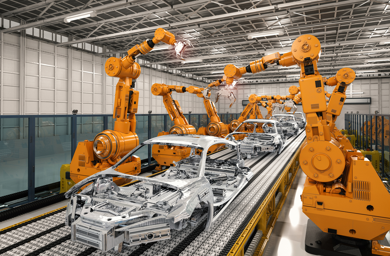
Imagine we want to train a ML model on identifying defective components during an industrial production pipeline. Hopefully, defects occur rarely; but this also means we have probably only a small number of images showing exemplary defects to train the network.
Using a GAN, we can generate additional images for any given defect type.
The data
We use the NEU surface defect database which contains 300 images of scratches on metal that occurred during production.
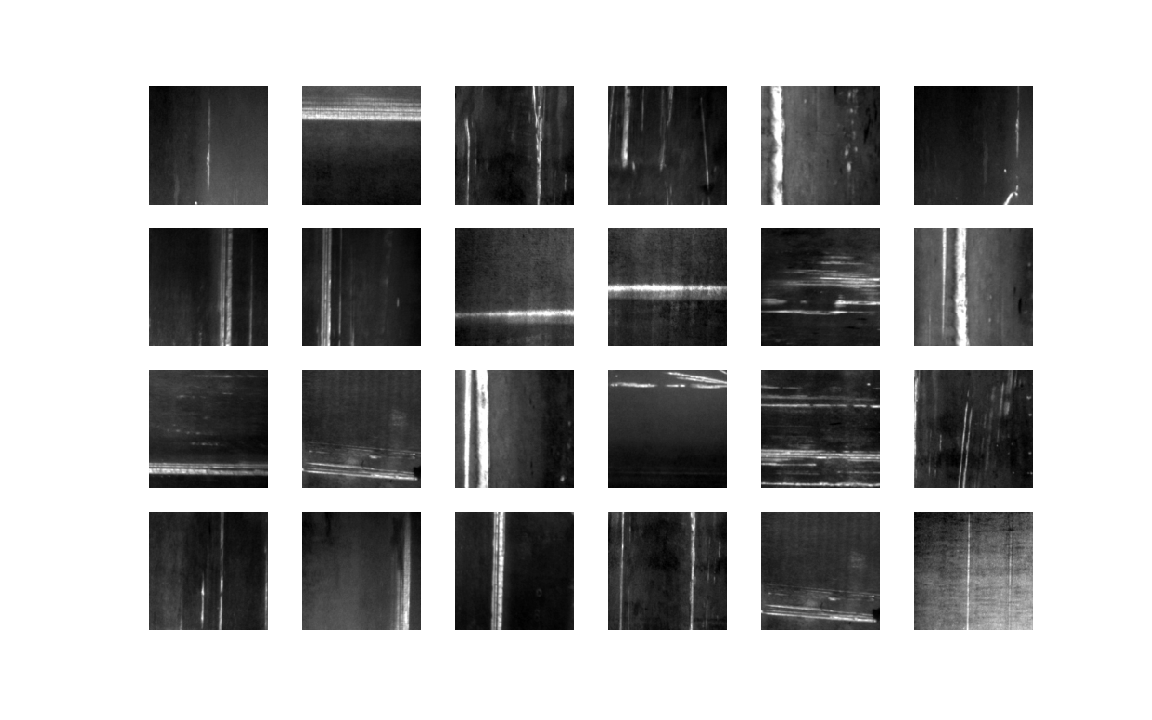
A GAN is an unsupervised learning method, so we don't need any labels. We do not have different kinds of labeled images we want to distinguish, rather we have a set of unlabeled data that we try to imitate.
The network
A GAN is not a single neural network. Rather, it combines two neural networks that play a game with each other. I will briefly explain the rules of the game.
How GANs work
First, there is a discriminator network, which is just a simple Convolutional Neural Network (CNN). Then we have the generator network, which is more or less a reversed CNN. It gets a random input and creates an image as output from up-sampling the input with transposed convolutions.
The game takes place as follows: The generator gets a random input and generates a picture. The discriminator takes alternately generated images and original images (without knowing which one is which) and tries to predict whether a given image is original or generated, taking into account only the features of the image.
Both networks try to get better over time. The discriminator attempts to distinguish the real images from the generated ones, while the generator aims to trick the discriminator into thinking its images are real.
.jpg)
Formally, the networks play this min-max game:
where
Here z is random noise activating the generator G to generate an image G(z). D is the discriminator that predicts whether an image is real or generated, i.e. D(x) is the probability that x is a real image. pdata is the distribution of the original data, pz the distribution of the noise.
So the discriminator tries to maximize its success, while the generator tries to minimize it. Here is a great a visualization of what happens when a GAN is trained. You might also like to check out this video:
The configuration
We use Python with PyTorch, some NumPy, Pandas and Matplotlib for visualizations. For the model we went with these configurations:
batch_size = 12
generator_depth = 64
discriminator_depth = 128 loss_function=nn.BCELoss()
number_of_epochs = 128
discriminator_optimizer = optim.Adam(discriminator.parameters(), lr=0.0004, betas(0.5,0.999))
generator_optimizer = optim.Adam(generator.parameters(), lr=0.0001, betas=(0.5,0.999))
In the following code block we define the discriminator, that gets the image as input. We define a sequence of filters the model uses to classify this input image. When we train it, we adjust these filters so that it learns to differentiate between original and generated images.
class Discriminator(nn.Module):
    '''
    The Discriminator that shall distinguish between dataset images and the ones generated by the generator.
    '''
    def __init__(self, number_of_gpus):
        super(Discriminator, self).__init__()
        self.ngpu = number_of_gpus

        self.layer1 = nn.Sequential(
            spectral_norm(nn.Conv2d(in_channels=3, out_channels=discriminator_depth,
                                    kernel_size=(4,4), stride=2, padding=1, bias=False)),
            nn.LeakyReLU(0.2, inplace=True)
        )

        self.layer2 = nn.Sequential(
            spectral_norm(nn.Conv2d(in_channels=discriminator_depth, out_channels=discriminator_depth*2,
                                    kernel_size=(4,4), stride=2, padding=1, bias=False)),
            nn.BatchNorm2d(discriminator_depth*2),
            nn.LeakyReLU(0.2, inplace=True)
        )

        self.layer3 = nn.Sequential(
            spectral_norm(nn.Conv2d(in_channels=discriminator_depth*2, out_channels=discriminator_depth*4,
                                    kernel_size=(4,4), stride=2, padding=1, bias=False)),
            nn.BatchNorm2d(discriminator_depth*4),
            nn.LeakyReLU(0.2, inplace=True)
        )

        self.layer4 = nn.Sequential(
            spectral_norm(nn.Conv2d(in_channels=discriminator_depth*4, out_channels=discriminator_depth*8,
                                    kernel_size=(4,4), stride=2, padding=1, bias=False)),
            nn.BatchNorm2d(discriminator_depth*8),
            nn.LeakyReLU(0.2, inplace=True)
        )

        self.layer5 = nn.Sequential(
            spectral_norm(nn.Conv2d(in_channels=discriminator_depth*8, out_channels=discriminator_depth*16,
                                    kernel_size=(4,4), stride=2, padding=1, bias=False)),
            nn.BatchNorm2d(discriminator_depth*16),
            nn.LeakyReLU(0.2, inplace=True)
        )

        self.output_layer = nn.Sequential(
            nn.Conv2d(in_channels=discriminator_depth*16, out_channels=1,
                                    kernel_size=(4,4), stride=1, padding=0, bias=False),
            nn.Sigmoid()
        )


    def forward(self, input_image):

        layer1 = self.layer1(input_image)
        layer2 = self.layer2(layer1)
        layer3 = self.layer3(layer2)
        layer4 = self.layer4(layer3)
        layer5 = self.layer5(layer4)
        return self.output_layer(layer5)
The generator has similar filters as the discriminator, just reversed. Instead of looking at the pictures to detect patterns, it returns images based on a pattern that we have taught it to draw. The input is a bunch of random numbers that activate those filters to draw an image.
class Generator(nn.Module):
    '''
    The Generator Network. It is mostly a reversed discriminator with a random input noise which outputs an image.
    '''
    def __init__(self, number_of_gpus):
        super(Generator, self).__init__()
        self.ngpu = number_of_gpus

        self.layer1 = nn.Sequential(
            nn.ConvTranspose2d(in_channels=100, out_channels=generator_depth*16,
                               kernel_size=(4,4), stride=1, padding=0, bias=False),
            nn.BatchNorm2d(num_features=generator_depth*16),
            nn.ReLU(inplace=True)
        )

        self.layer2 = nn.Sequential(
            nn.ConvTranspose2d(in_channels=generator_depth*16, out_channels=generator_depth*8,
                               kernel_size=(4,4), stride=2, padding=1, bias=False),
            nn.BatchNorm2d(num_features=generator_depth*8),
            nn.ReLU(inplace=True)
        )

        self.layer3 = nn.Sequential(
            nn.ConvTranspose2d(in_channels=generator_depth*8, out_channels=generator_depth*4,
                               kernel_size=(4,4), stride=2, padding=1, bias=False),
            nn.BatchNorm2d(num_features=generator_depth*4),
            nn.ReLU(inplace=True)
        )

        self.layer4 = nn.Sequential(
            nn.ConvTranspose2d(in_channels=generator_depth*4, out_channels=generator_depth*2,
                               kernel_size=(4,4), stride=2, padding=1, bias=False),
            nn.BatchNorm2d(num_features=generator_depth*2),
            nn.ReLU(inplace=True)
        )

        self.layer5 = nn.Sequential(
            nn.ConvTranspose2d(in_channels=generator_depth*2, out_channels=generator_depth,
                               kernel_size=(4,4), stride=2, padding=1, bias=False),
            nn.BatchNorm2d(num_features=generator_depth),
            nn.ReLU(inplace=True)
        )

        self.output_layer = nn.Sequential(
            nn.ConvTranspose2d(in_channels=generator_depth, out_channels=3,
                               kernel_size=(4,4), stride=2, padding=1, bias=False),
            nn.Tanh()
        )


    def forward(self, input_noise):

        layer1 = self.layer1(input_noise)
        layer2 = self.layer2(layer1)
        layer3 = self.layer3(layer2)
        layer4 = self.layer4(layer3)
        layer5 = self.layer5(layer4)
        return self.output_layer(layer5)
The training
We can split the training into three parts.
Training the discriminator with real images:
discriminator.zero_grad()

prediction = discriminator(batch)

labels_for_dataset_images = torch.ones((batch_size,), device=device).view(-1)

loss_discriminator = loss_function(prediction.view(-1), labels_for_dataset_images)
loss_discriminator.backward()
Training the discriminator with the generated images from the generator:
random_noise = torch.randn(batch_size,100,1,1, device=device)
generated_image = generator(random_noise)

labels_for_generated_images = torch.zeros(np.prod(prediction.size()), device=device)

prediction = discriminator(generated_image.detach())

loss_generator = loss_function(prediction.view(-1), labels_for_generated_images)
loss_generator.backward()

discriminator_optimizer.step()
Training the generator:
generator.zero_grad()

prediction = discriminator(generated_image).view(-1)

loss_generator = loss_function(prediction, labels_for_dataset_images)
loss_generator.backward()

generator_optimizer.step()
Results
Are we just regenerating the images from the data set?
If the generator overfits, we could obtain images that are very similar or even almost the same as images from the data set. This of course is not the result we want. So we test how similar our generated images are to the images in the data set.
I use the k-nearest-neighbour approach. This is a classification algorithm which searches for the "nearest" images from the image it wants to classify to all images in the data set.
In our case, calculating the distance means considering every pixel as a dimension and then just calculating the euclidean distance between these (128x128)-dimensional images.
Let's have a look at the nearest or most similar images from the original data set for some of our generated images:
def euclidean_distance(a, b):
    '''
    Calculates the euklidean Distance of two torch tensors of the same size.
    '''
    return torch.sqrt(((a - b) ** 2).sum())


def get_k_nearest_samples(image, k):
    '''
    Searches for the k-nearest samples in the dataset of a given image based on the euclidean distance.
    '''
    return np.argsort([euclidean_distance(image[0][0], sample[0][0]) for sample in dataset])[:k]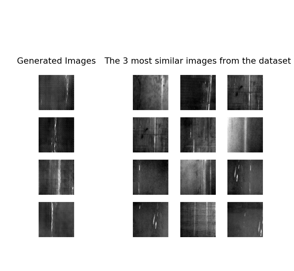
The images are similar to the data set images, but they are not too similar - so the generator didn't overfit.
Conclusion
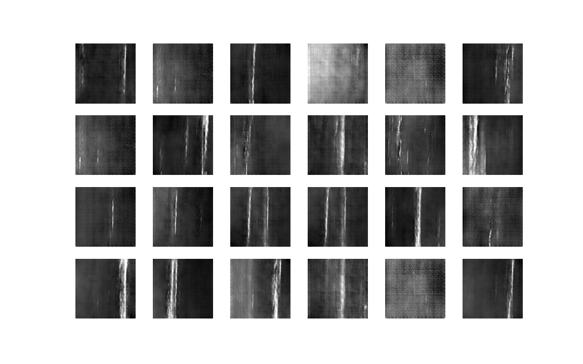
The Generative Adversarial Network has indeed learned how to generate new images from the given data distribution: They are genuinely new, because they are not just copies of the original images, and still can't be distinguished from the original ones. Thus we could use these newly created images to train a defect detection or defect classification model.
Of course, in practical situations you should always double-check that the GAN-created images really have a positive impact on the model performance. This might not always be the case.
Having said that, there are a lot of potential use cases for GANs (not only) in industrial production. Due to the current research interest in GANs we will have a lot of new insights about when and how to use them very soon.
At last, a little warning: Tuning GANs is pretty annoying and small changes can lead to distorted outputs. Moreover, training them is a computationally expensive task, because you have to train two networks at once. You won't get far without a strong GPU.
Would you like to read about related projects? You can have look at one here: Automatic Defect Detection in Production.
Contact
If you would like to speak with us about this topic, please reach out and we will schedule an introductory meeting right away.