BERT for question answering (Part 1)

BERT is a deep learning model for language representations and serves as a pretraining approach for various NLP problems (so called downstream tasks). Specific applications are for example Named Entity Recognition, Sentiment Analysis and Question Answering. You can find the official paper proposing BERT here.

The main idea of BERT is to perform an unsupervised pretraining phase on a large generic text corpus(such as Wikipedia articles or book collections) in order to learn reasonable language representations.

During a fine-tuning phase, the previously learned representations are used as a baseline for a problem-specific training.

From BERTs git repo:

Pre-training is fairly expensive (four days on 4 to 16 Cloud TPUs), but is a one-time procedure for each language (current models are English-only, but multilingual models will be released in the near future). We are releasing a number of pre-trained models from the paper which were pre-trained at Google. Most NLP researchers will never need to pre-train their own model from scratch. Fine-tuning is inexpensive. All of the results in the paper can be replicated in at most 1 hour on a single Cloud TPU, or a few hours on a GPU, starting from the exact same pre-trained model. SQuAD, for example, can be trained in around 30 minutes on a single Cloud TPU to achieve a Dev F1 score of 91.0%, which is the single system state-of-the-art.

The core components of BERT are bidirectional transformers, which were originally proposed in this paper.

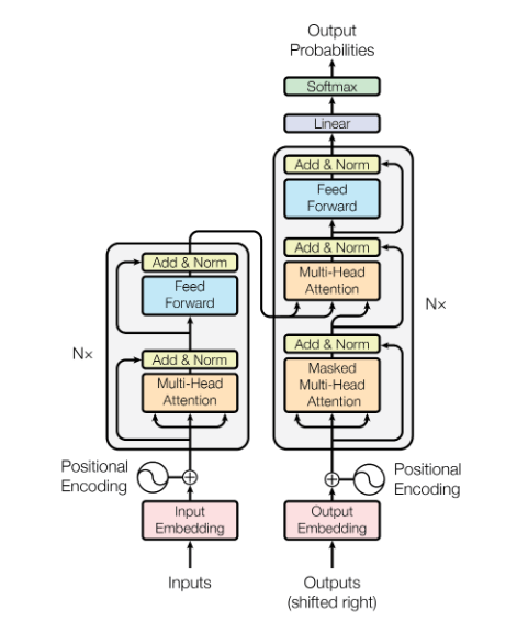
The architecture (encoder on the left, decoder on the right) of the original transformer is shown in the image below. Note that the terms "encoder" and "decoder" are interpreted in a slightly different way compared to for example commonly used convolution neural networks: we do not have the typical "encoding" in the sense of layers getting narrower and the typical "decoding" in the sense of layers getting wider (like for example in an autoencoder network). Instead, the decoder consumes model outputs of previous sequence components as an input: this distinguishes both components of the network.

Through the whole model, you find so-called residual connections (original paper here), which skip the attention layers (see below for an explanation of the attention mechanism) and feed the output of a previous layer directly into an addition layer including a layer normalization (original paper here). A comprehensive introduction to transformers including PyTorch code can be found here.

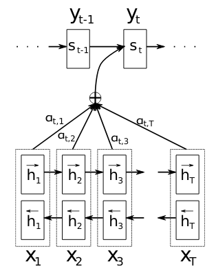
Transformers make use of the so-called attention mechanism, which was proposed in this paper in the context of machine translation. The idea of the attention mechanism is to obtain every decoder output as a weighted combination of all the input tokens. Prior to this approach, most NLP tasks based on RNNs usually obtained an output from a single aggregated value of all the previous objects in the input sequence. This is quite a big problem especially for long input sequences, since information at the end of the input sequences compresses all prior sequence components, thereby potentially introducing a lot of noise. See the visualization of the attention mechanism (in this case with a bidirectional RNN) from the original paper here:

The idea is that the encoding-decoding process based on the attention mechanism now performs the particular task (such as translation) in combination with an "alignment search", i.e. it additionally learns how each one of individual input sequence components is involved in the resulting output sequence instead of just going through a prescribed output order via "classical" end-to-end RNN decoding. This operation is visualized in the figure above in terms of the weights $$\alpha_{t,i}$$, which determine the influence of the $$i$$-th input component on the $$t$$-th output component (again, in this case with a bidirectional RNN model instead of the transformer which is used in BERT).

For the case of the transformer, multiple attention layers are stacked in order to obtain the encoder and decoder structures.

The original implementation of BERT comes in two model sizes: a BERT base model with a hidden middle layer size of $$H=768$$ dimensions and a BERT large model with a hidden layer size of $$H=1024$$ dimensions. The encoder/decoder blocks consist of $$12$$​ and $$24$$ layers of transformers, respectively. All layers contained in the model have the same size - note that this is also needed for the residual connections.

The raw BERT model can take either a single sentence or two sentences (which we will call input segments/sentences ​ and ​ in what follows) as a token sequence input, which makes BERT flexible for a variety of downstream tasks. The ability to process two sentences can for example be used for question/answer pairs. BERT comes with is own tokenization facility.

As an input representation, BERT uses WordPiece embeddings, which were proposed in this paper. Given a vocabulary of ~30k word chunks, BERT breaks words up into components - resulting in a tokenization $$[t_1, \dots, t_l]$$ for an input sequence of length $$l$$. We will have a closer look at the tokenization below. An exploration of BERTs vocabulary can be found here.

WordPiece is a language representation model on its own. Given a desired vocabulary size, WordPiece tries to find the optimal tokens (= subwords, syllables, single characters etc.) in order to describe a maximal amount of words in the text corpus.

The important part here is that WordPiece is trained separately from BERT and basically used as a black box to perform vectorization of input sequences in a fixed vocabulary. This procedure will be performed for every word in the input after a general string sanitizing. The catch of the WordPiece idea is that BERT can represent a relatively large catalog of words with a vector of fixed dimension corresponding to the vocabulary of chunks. There are several ways to deal with out-of-vocabulary tokens, see the original WordPiece paper linked above. The tokens generated by WordPiece are usually mapped to IDs in the corresponding vocabulary to obtain a numerical representation of the input sequence. These IDs are typically just the number of the index in the vocabulary list (however, it is also possible to use hash functions on the tokens). It is actually fairly easy to perform a manual WordPiece tokenization by using the vocabulary from the vocabulary file of one of the pretrained BERT models and the tokenizer module from the official BERT repository.

The characters ## indicate that the token is associated with the previous token (for example by breaking up a single word into tokens). In BERTs case, the numerical representation of the tokens is just the mapping to their indices in the vocabulary:

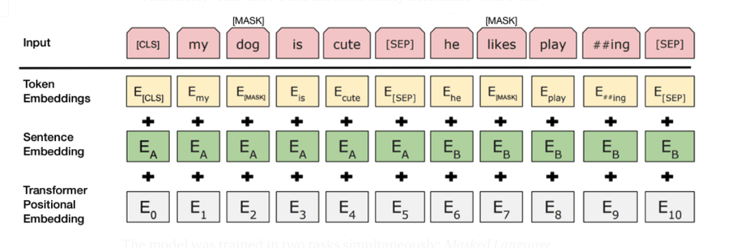
In case two sentences are passed to BERT, they are separated by using a special [SEP] token. All inputs start with a [CLS] token, which indicates the beginning of a token sequences and is later used as a representation for classification tasks (see the pretraining section below).

The token embeddings will be compared to word embedding lookup tables and become the so-called token input embedding $$E_{ti} \in \mathbb{R}^H$$ (again, $$H$$ is the dimensionality of the hidden layers of BERT as introduced above). Interestingly, besides the "flat" token mapping to their IDs, a one-hot encoding version of the tokens is also contained in BERTs source code.

Assuming that we have now obtained the token embeddings $$E_{ti}$$ (that is, word embeddings generated from either a mapping of tokens to IDs or a one-hot encoded version), a learned sentence embedding $$E_A \in \mathbb{R}^H$$ or $$E_B \in \mathbb{R}^H$$  is added, depending on the sentence which the token belongs to.

As a third information, BERT uses an embedding of the token position in the input sequence: the positional embedding $$E_i \in \mathbb{R}^H$$ corresponding to token $$t_i$$. Positional embeddings are vectors of the same size as the other two embeddings. The positional embedding is needed since BERT itself does not have an intrinsic sequential ordering like for example a recurrent neural network. In the original paper which proposed the so called transformer layer (see section below) a embedding rule in terms of a vector consisting of sinusoids was proposed. In particular, let $$E_{i,j}$$ denote the $$j$$-th entry of the positional encoding vector $$E_i \in \mathbb{R}^H$$ related to the token $$t_i$$. Then the embedding rule used in the original transformer paper is

as well as

for all $$ 1 \leq j \leq \lfloor{H/2}\rfloor$$.

Learning the positional embeddings has also been proposed. The original BERT paper does not elaborate on which positional embedding is chosen. However, it is mentioned that the implementation is based on the paper introducing the transformer layer.

For every input token $$t_i$$, the token embedding $$E_{ti}$$ the positional embedding $$E_i$$  and the corresponding sentence embedding vector $$E_A/E_B$$ are then summed up in order to obtain the final input embedding representation for of the $$i$$-th input for BERT.

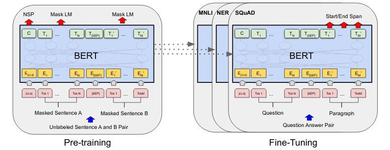
By propagating this input representation through the full model we will then obtain the final hidden embedding $$T_i \in \mathbb{R}^H$$ from the token $$t_i$$ (see the image in the section below).

Pretraining of BERT is performed in an unsupervised manner on fairly large unlabeled text corpora (such as Wikipedia articles). The original BERT version was trained on the BooksCorpus and English Wikipedia. During the pretraining phase, BERT performs two particular tasks:

1. Masked Language Modeling:

In order to learn the connection between smaller text components such as words and tokens, tokens of the input sequences are chosen at random (15% of the original input sequence tokens). Among these selected tokens, a word replacement routine with a [MASK] token is performed. In order to not introduce a model bias towards the mask token, a small percentage of the selected tokens are replaced with a randomly chosen token or remain unchanged. The hidden representation of the input tokens will then be used in combination with a softmax classifier in order to predict the selected tokens from BERTs vocabulary under a cross entropy risk.

2. Next Sentence Prediction:

This task is performed in order to learn connections between sentences. From the available text corpora, sentence pairs are formed. Whenever the pairs are subsequent in the original text, a IsNext label is attached to them. Whenever the sentence pairs are not subsequent in the original texts, a NotNext label is attached. The training dataset is generated of 50% pairs with IsNext label and 50% NotNext label. BERT now predicts the two labels as a binary classifier based on the hidden layer embedding of the [CLS] token of the input sequence. The left side of the image below visualizes how the hidden representations $$C \in \mathbb{R}^H$$ and $$T_i \in \mathbb{R}^H$$ of the [CLS] token and the text segment token $$t_i$$ are used for these tasks.

Fine-tuning of BERT is always associated with a particular practical task such as for example classification. The pretraining version of BERT (that is, the weights obtained from the Masked Language Modeling and Next Sentence Prediction training routines outlined above) are used as starting weights for a supervised learning phase.

Depending on the specific task, various components of BERTs input can be used. For a text sequence classification task, the representation of the [CLS] token will be used. For tasks involving two sentence inputs such as paraphrasing and question/answer problems, we make use of the sentence $$A$$/$$B$$ mechanism described in the previous sections.

Usually, additional neurons/layers are added to the output layer of BERT: in the classification case this could for example be a softmax output. Given a training data set, a standard end-to-end training routine for the full BERT model with the task-specific modified output layers is run. Typically, the fine-tuning phase is a much faster procedure than the pretraining phase, since the transfer from Masked Language Modeling and Next Sentence Classification to the particular fine-tuning task allows to start from a near-converged state.

That's it for the first part of the article. In the second part we are going to examine the problem of automated question answering via BERT. You can also read about a project we did for idealo, where we used different BERT models for automatic extraction of product information.

• A Neural Named Entity Recognition and Multi-Type Normalization Tool for Biomedical Text Mining; Kim et al., 2019.

• Attention Is All You Need; Vaswani et al., 2017.

• BERT: Pre-training of Deep Bidirectional Transformers for Language Understanding; Devlin et al., 2018.

• BioBERT: a pre-trained biomedical language representation model for biomedical text mining; Lee et al., 2019.

• Google’s Neural Machine Translation System: Bridging the Gap between Human and Machine Translation; Wu et al., 2016.

• Neural machine translation by jointly learning to align and translate; Bahdanau et al. 2015.

• Pre-trained Language Model for Biomedical Question Answering; Yoon et al., 2019.

• Real-Time Open-Domain Question Answering with Dense-Sparse Phrase Index; Seo et al., 2019.

• The Annotated Transformer; Rush, Nguyen and Klein.