X-ROCKET to the moon

Felix Brunner

February 15th 2024

These are the voyages of the encoder model X-ROCKET. Its continuing mission: to explore strange, new time series; to seek out new explanations and new interpretations; to boldly seek meaning where no one has sought before. Previously in this series, we completed our training in the basics of time series classification in part one and learned how to operate X-ROCKET in part two. But enough with all the talking, it is time to fire up the X-ROCKET engines and see this model in action. Let’s rocket!

Data, prepare for takeoff!

We will use the “AsphaltPavementTypeCoordinates” dataset from Souza (2018) as an example. This dataset consists of 2,111 examples of accelerometer data recorded from cars passing over various types of pavement. Every time series example in the dataset has three channels (corresponding to the X, Y, and Z directions), each of which is measured at 100 Hz. The length of recordings varies from 66 time observations up to 2,371. The classes are “flexible” (38.6%), “cobblestone” (25.0%), and “dirt road” (36.4%). According to the description, the best model achieved an accuracy of 80.66% on this task, which we will use as a benchmark. So, Houston, we have our problem — a relatively balanced three-way multivariate time series classification problem, to be precise.

The aeon module provides a simple way to load this dataset for our machine learning task. We will also use scikit-learn to follow the original authors and divide the full dataset into equally-sized train and test splits:

from aeon.datasets import load_classification
from sklearn.model_selection import train_test_split

X, y, meta = load_classification("AsphaltPavementTypeCoordinates")
X_train, X_test, y_train, y_test = train_test_split(
    X, z, test_size=0.5, random_state=0
)

How to build a ROCKET

Next, let’s put together a suitable vessel to encode this dataset. Having installed the xrocket module with its dependencies in our environment, we can immediately import the full encoder module. Then, all we have to do is initialize an instance of it with suitable parameters for our problem. Since our dataset has three channels the choice of in_channels is clear. Next, as the time series length varies widely within our dataset, it makes sense to set max_kernel_span to a value suitable also for the shorter examples, let’s do 100 in this case. Finally, we leave combination_orderand feature_cap at its default values of one and 10,000 for now:

from xrocket import XRocket

encoder = XRocket(
    in_channels=3,
    max_kernel_span=100,
    combination_order=1,
    feature_cap=10_000,
)

Given these inputs, our encoder is automatically set up to have the usual 84 MiniROCKET kernels at 12 distinct dilation values. With three data channels, X-ROCKET chooses to use three pooling thresholds for each kernel-dilation-channel combination to stay within the feature_cap. Hence, the embedding dimension is 84 12 3 * 3 = 9,072. To finally prepare this contraption for boarding, all we have to do is find suitable values for the 9,072 pooling thresholds. We do this by fitting our XRocket instance to a data example. As the model operates on PyTorch tensors, where the first dimension is reserved for stacking multiple examples in a batch, all we have to do is transform the data from a 2D numpy array into a 3D tensor and feed it to the encoder:

from torch import Tensor

encoder.fit(Tensor(X_train[0]).unsqueeze(0))

Punch it!

Now that our X-ROCKET is calibrated, let’s start the countdown. Again, inputs need to be in the 3D tensor format, so we need to transform the examples to PyTorch tensors before passing them to the model. Due to the varying time series lengths, we can not concatenate multiple examples into a batch so easily. Therefore it is more convenient to encode the examples one by one and collect the embeddings in two lists, one for the training set and one for the test set. Time to go to full thrust, godspeed!

embed_train, embed_test = [], []
for x in X_train:
    embed_train.append(encoder(Tensor(x).unsqueeze(0)))
for x in X_test:
    embed_test.append(encoder(Tensor(x).unsqueeze(0)))

8.02 seconds on a moderately fast consumer-grade CPU later, the embeddings of both the train and the test set are ready. That is, we now have a representation of the varying-size input data in fixed-dimensional vectors. Hence, the time has come to make this a tabular problem with named features stored in a DataFrame. The encoder provides the attribute feature_names that readily contains the names of each embedding value as a tuple of (pattern, dilation, channel, threshold). Let’s put these tuples in an index and name them accordingly. Then finally, we create the frames to store the transformed datasets. Who said time series classification had to be rocket science?

from torch import concat
import pandas as pd

feature_names = pd.Index(encoder.feature_names)
df_train = pd.DataFrame(data=concat(embed_train), columns=feature_names)
df_test = pd.DataFrame(data=concat(embed_test), columns=feature_names)

Giving X-ROCKET a purpose

As with so many things in the universe, X-ROCKET struggles to find its way without a head. To make sure it can follow its trajectory to the intended destination — time series classification — let’s find a suitable prediction head that delivers the payload. As mentioned before, any prediction model that fits the intended purpose is fine in principle. Note that in theory, this also includes deep PyTorch feed-forward neural networks, which allow to run backpropagation end to end back to the X-ROCKET weights to improve its embeddings. But don’t panic, it is possible to find answers even without Deep Thought! Since we are eventually interested in the explainability of the predictions, let’s pick a simple and explainable classification model instead. Scikit-learn’s RandomForestClassifier is a solid start on that end, all we have to do is load it and fit it on our training data:

from sklearn.ensemble import RandomForestClassifier

clf = RandomForestClassifier(random_state=0)
clf.fit(df_train, y_train)

Wow, it almost went off like a rocket! Just 3.13 seconds later, we have our classifier. Let’s see how it does on the dataset. Since the original work claims to achieve 80.66% accuracy, let’s score our model in the same way on the hold-out set as they did:

from sklearn.metrics import accuracy_score

pred_test = clf.predict(df_test)
acc_test = accuracy_score(y_test, pred_test)

And there we have it, our model achieves an accuracy of 90.19% on the test set! Not bad, but is it enough to make a little rocket man proud? To conclusively answer that question, of course, more rigorous comparisons are warranted. Nevertheless, this appears to have been a successful launch!

Where no ROCKET man has gone before

The time has come to take X-ROCKET to the final frontier on its ultimate quest for meaning. Since the model seems to work acceptably well, it is valid to also analyze the explanations it provides about its predictions. Luckily, the random forest classifier we chose provides an attribute called feature_importances_, which ascribes importance scores to all features of the model. Since we have stored the corresponding index in feature_names, we can easily bring together both arrays:

feature_importances = pd.Series(
    data=clf.feature_importances_,
    index=feature_names,
)

As it is, analyzing this object is only so useful. For example, we can see that the most important embedding for our model is the pattern HLHLLLHLL at dilation two in the Y-channel with pooling threshold of -10.84. An H in the pattern indicates a high value, while an L indicates a low such that the pattern looks something like |_|___|__. However, it is now easy to pool importance values to examine the relative importances of, say, the input channels. Summing over each channel we get the importance scores below. Given the way X-ROCKET removes the randomness in the way the embeddings are put together, the same features are extracted from each channel and each dilation value. Hence, comparing grouped feature importances this way offers a fair comparison.

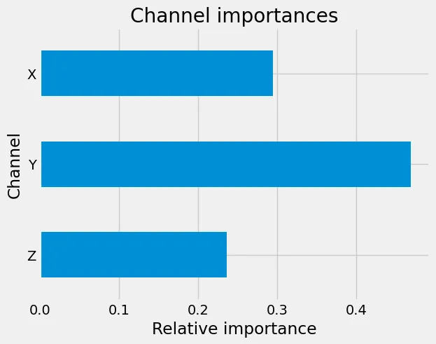
Relative importances of the input channels for the predictions.

That is, the Y-channel seems to be the clear favorite, followed by the X-channel. Similarly, if we sum over the various dilation values, a clear insight is that higher frequencies are the ones that matter. With entries being recorded at 100 Hz, a dilation value of 2 means a frequency of 50 Hz, for example. As can be seen in the image below, most information is contained in these higher frequencies, that is, the ones with smaller dilation values.

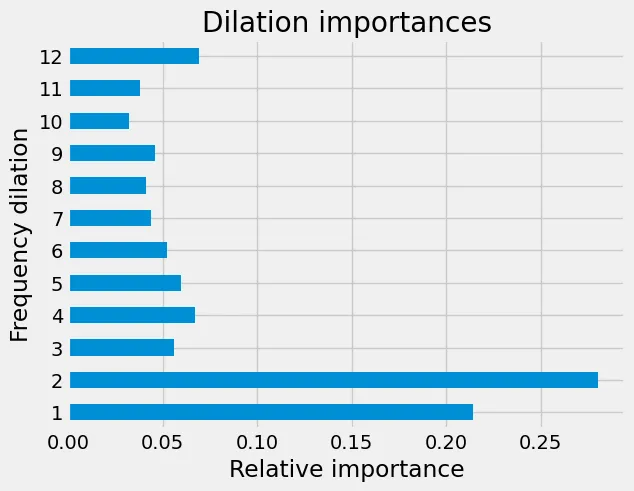
Relative importances of various frequency dilations for the predictions.

What did the doctor say to the ROCKET?

“Time to get your booster shot!” Accordingly, one might wonder what could be ways to provide an extra performance boost to this rocket ship. In machine learning space, of course, the possibilities are endless. For example, one could try alternative model heads such as gradient boosting algorithms, or better optimize the corresponding hyperparameters. On a different route, one could think about how to improve the data quality or augment the existing dataset with artificial examples. However, this is beyond the scope of this simple demonstration. What would be interesting to see though, is if the encoder can be further improved to gain additional insight into the drivers of predictiveness when also considering multi-channel features besides the previously seen univariate ones. So let’s leave everything unchanged, but only alter the encoder by setting combination_order=2 and increase the number of features slightly with feature_cap=15_000 when initializing X-ROCKET. The resulting embedding is now 12,096-dimensional with 6 channel combinations instead of only the 3 channels, and 2 pooling thresholds for each output.

Besides a slight increase in test set accuracy to 91.13%, we again observe that the Y-channel again seems to be the most important, but now combinations of Y with the other channels carry increased importances:

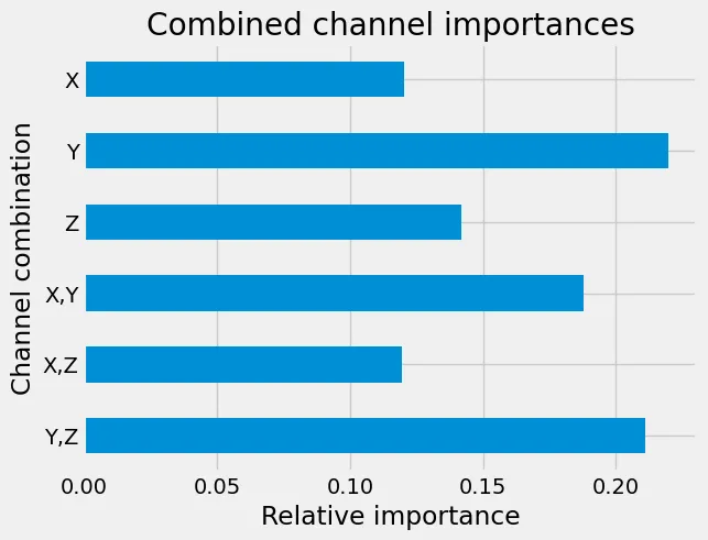
Relative importance of input channel combinations for the predictions.

Conclusions

In this series of articles, we have seen how an existing time series encoder framework can be restructured to derive new insight into the prediction drivers. Part one has shed light on some of the advances in machine learning for the time series domain. Then, part two and this third part presented X-ROCKET, an explainable time series encoder, both technically and with a practical usage example. While this construct has completed its mission in the example here, it is important to point out that the explanations provided by X-ROCKET are only as good as the model’s prediction capabilities on the respective problem. That is, there is no point in interpreting a model that does not perform well enough in terms of its predictions. Hence, there is no guarantee that the same approach works equally well in different settings, in particular, if there is little signal in the input data. Nonetheless, rockets are cool, there is no getting around that!

References

Dempster, A., Schmidt, D. F., & Webb, G. I. (2021, August). Minirocket: A very fast (almost) deterministic transform for time series classification. In Proceedings of the 27th ACM SIGKDD conference on knowledge discovery & data mining (pp. 248–257).
Souza, V. M. (2018). Asphalt pavement classification using smartphone accelerometer and complexity invariant distance. Engineering Applications of Artificial Intelligence, 74, 198–211.

This article was created within the “AI-gent3D — AI-supported, generative 3D-Printing” project, funded by the German Federal Ministry of Education and Research (BMBF) with the funding reference 02P20A501 under the coordination of PTKA Karlsruhe.